Marginal productivity theory of wages Assumptions, Diagram

Marginal productivity theory of wages

            Economists David Ricardo and west first of all propounded the concept of marginal productivity. Both Ricardo and west applied the marginal productivity principle only to land. But the idea of marginal productivity did not gain much popularity till the last quarter of 19th century. After that the economists like J.B. Clark, Jevons, Wicksteed, Walr as have popularized this theory, Modern time, Prof. Alfred Marshall.

            J.R. Hicks have popularized the doctrine of marginal productivity.

            Originally, this theory was developed to explain the determination of wage but later the theory was also used to explain the determination of the reward of other factors of production such as Land, Capital and Organization Simultaneously.

            Though this theory is explained with respect to wage determination, the theory is also applicable in the context of other factors; hence this theory is called general theory of distribution.

            Every worker has capacity to produce some goods and services, for such capacity, an employer in any company hire him. So, the company pays him according to his capacity to produce. Hence, the marginal productivity theory tells us how much the remuneration of a factor is.

            In another word, a factor of production should be paid according to the contribution made by it to the total production. Thus, it is clear that under marginal productivity theory, the price of each factor of production is fixed just equal to its marginal productivity. There are two important versions of this theory such as J.B. Clark's version and Marshall. Hicks Approach.

            Marginal productivity theory: Clarkian Version Clarkian version of marginal productivity. Theory is based on the following assumptions.

(i)   Constant population

(ii)  Constant amounting of capital

(iii) Constant technique of production

(iv) There is perfect competition in the factor market

(v)  Labor is homogeneous & perfectly mobile.

(vi) Society is completely static.

            Every rational employ or entrepreneur will try to utilize his existing amount of capital so as to maximize his profits. For this, he will hire as many laborers as can be profitably put to work with the given amount of capital. For an individual firm or Industry, marginal productivity of Labor (MPC) will decline as more and more laborers are added to the fixed quantity of capital factor.

            Marginal productivity means the charge in the amount of total output as a result of hiring an additional unit of Labor or marginal productivity means per man productivity. An entrepreneur will go one hiring the Labor up to that point where marginal productivity is greater than the current wage rate. Therefore, the entrepreneur will reach at the equilibrium position when wage rate equals to the marginal productivity of labor, because in this condition his profit will be maximized. The equilibrium condition under Clarkian version is explained below.

            In the figure below, marginal productivity (MP) and number or amount of labor units are expressed on OY and OX axes respectively. The curve MP represents the marginal productivity of labor employed on the production process. Here, in the figure below, NP curve shows the diminishing marginal product of labor.

            Here, is the figure, OW is the prevailing wage rate. Now it will be profitable for the employer to employ units of labor since the marginal productivity of labor is equal to prevailing wage rate OW. Hence Employer would not employ more than OL amount of labor as the marginal product of labor will fall below the wage rate OW and he will be in loss.

            Since It is assumed that in the labor market, there is perfect competition, then an individual firm or industry will haze no control over the wage rate. Thus, an individual firm or industry has to decide only at what amount of labor, about the amount of labor, to be hired at the work at prevailing wage rate to get maximum profit.

            From the above explanation, it is not clear that how the prevailing wage rate is determined. To explain this, Clark, has taken the example of whole economy where he assumed that all the available laborers have Job i.e. assumption of full employment of labor prevails in the economy.

            Now, wage rate determination can be demonstrated by the following figure.

            In this figure, MP curve shows diminishing marginal product of labor. Suppose. In the whole economy the total labor is available to OL quantity and their marginal productivity equal to CD, which is equal to OW wage rate became the total marginal product of all the laborers' is equal to the wage rate aw, we have to examine, how it is determined. Suppose, if wage rate s increased from OW to OW1 then labor employment will declare to OL, remaining L₁L number of unemployed laborers in the economy. Due to competition among the laborers to get Job, they influence the wage rate and it reduced to OW wage rate. Contrary to this, if wage, rate decreases, from OW to OW_2, the producer will tend to employ more laborers equal to OL₂ but in the economy the total labor is available only to OL units. Hence, due to scarcity of labor force, employer will increase wage rate to attract the laborers. As a result again wage rate will be determined at OW. Hence, It is clear that the wage rate of labor is determined equal to the amount of marginal productivity of labor found in the whole economy. Hence, the wage rate OW is equal to marginal productivity of OL units of labor.

            Marshall-Hicks marginal productivity theory. Clarkian version of marginal productivity could not explain the supply side of labor. According to Clark, Demand side is only the determinant for the determination of wage rate or under his version of marginal productivity theory.

            It is only clear that how much an entrepreneur at different level of wage will make demand of labor rates in the economy, or according to Clarkian version. Marginal productivity only determines the demand of factor.

            According to Marshall and Hicks, wage rate is determined by both demand & supply sides. The wage rate determined by demand and supply will be equal to the marginal productivity of labor employed at the work.

            According to Marshall, marginal products do not determine wages; marginal products are determined to gather with the wage [i.e. price of a factor] by the interaction of demand and supply.

            Demand curve of labor derived under the marginal productivity concept is down ward sloping from left to right. This means with the additional unit of labor employed in the production, the marginal productivity of that factor decreases supply curve of labor will be upward sloping because of the positive relation between wage rate and labor supply. Generally with higher rate of wage, there will be more laborers encouraged to work and with the lower rate of wage, there will be lower level of supply of laborers with the interaction between demand and supply. The wage rate determination is explained below.

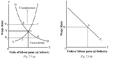
            From the figure, point 'E' is the [from (a) pane], equilibrium point where demand D and supply Ss cut, each other. OW and the corresponding labor employed in the industry are equal to OJ. Suppose if wage rate increases from on to OW_1, there will be excess supply of labor this means there will be unemployment shown in the figure (in panel P). Because there is W₁R total labor demand where the total supply is W₁T and the labor supply is excess than labor demand by RT. Hence, due to more supply of labor. Laborers will complete for looking Job and wage rate will come for looking Job and wage rate will come down to the equilibrium level at OW.

            Again, if wage rate decreases from OW to OW₂ there will be excess demand by JK amount of labor because here total labor demand is W₂ K and total labor supply is equal to W₂J, which is smaller than total demand. Due to the excess demand of labor, created by the employers, there will be competition among them and wage rate will again reach to OW then which is the equilibrium wage rate at this level of wage. Hence the corresponding employment labor is equal to OJ unit.

            Here, it is cleat that the wage rate OW determined by the interaction between demand and supply of labor is equal to the marginal productivity of labor employed in the economy, This has been explained by the panel (b). With given wage rate OW, the firm will employ the labor equal to OL units where wage rate (OW) is equal to marginal productivity of labor (MPL) at point E. Hence, at this level of wage rate I firm employs its labor will make maximum profit. Thus, Marshall Clark’s version of marginal productivity of labor as the former can describe the process of wage rate determination.